Using R Analytic Functions in PostGIS
This is the third and final post of the series intended to introduce PostgreSQL users to PL/R, a loadable procedural language that enables a user to write user-defined SQL functions in the R programming language. The information below provides sample use of R Functions against the NDVI dataset.
As introduced in the previous posts, the combination of PostgreSQL and R provides users with the ability to leverage the power and efficiency of PostgreSQL and the rich analytic functionality of R. When further combined with PostGIS, the geospatial extender for PostgreSQL, users can perform powerful spatial analytics within the PostgreSQL database. It is our hope that these posts will cause those building analytic applications to give PostgreSQL a second look.
The first post in this series provided users with an introduction, and discussed acquisition of administrative area boundary polygons (USA states and counties) and geocoding. The second post in this series worked through preprocessing of Normalized Difference Vegetation Index (NDVI) satellite raster data in preparation for spatial analytics.
Example Overview and Setup
This series of posts uses NDVI data from the moderate-resolution imaging spectroradiometer (MODIS) made available by the United States Geologic Survey (USGS). This data is used to demonstrate R analytic operations in PostgreSQL and PostGIS:
- Determining Average NDVI for a Particular Location Over Time
- Visualize Average NDVI for a Particular Location Over Time with
ggplot - Visualize Average NDVI for a Particular Location by Month
- Visualize Same Month Average NDVI for a Particular Location by Year
For information regarding the background for this analysis and the example set up, please take a moment to review the initial post in this series.
Analytics Operations
Having previously preprocessed and ingested the data from our example, it is now possible to perform a wide variety of R analytic functions against the data. This post works through a few examples of potential analysis as well as the resulting graphical output.
Determining Average Over Time
As an initial example of capability, we will use PL/R functions to determine the
average NDVI for San Diego county as a function of time. In order to perform
this analysis, first create a new function that reads the named geotiff file in
which the preprocessed raster layers were stored. These layers correspond to
different snapshots in time, from the year 2000 through 2016, for the NDVI
values for San Diego county. The commands below create this function that is
referred to as get_ndvi_mean().
This newly created function get_ndvi_mean() reads in the raster layers, and
then for each layer calculates the grand average for the entire county based on
the cell (pixel) level values. It combines those average county NDVI values with
their corresponding average acquisition date using the method described in the
previous post, and returns the results as one row per layer date and layer
average pair.
The average NDVI for San Diego county as a function of time can be determined
using the get_ndvi_mean() function described above by executing the following
commands:
CREATE OR REPLACE FUNCTION get_ndvi_mean
  (rastfile text, OUT lyr_date date, OUT lyr_mean float8)
RETURNS setof RECORD AS $$
  library(sp)
  library(raster)

  # read preprocessed NDVI data
  ndvi <- brick(rastfile)
  # calculate layerwide-mean per layer
  ndvi_mn <- cellStats(ndvi, stat = 'mean')

  # read layer dates
  conn <- dbConnect(dbDriver("PostgreSQL"), user="postgres", dbname="gis", host="localhost")
  sql.str <- "SELECT lyr_date FROM ndvi_dates(get_robj('ndvi_dt'))"
  ndvi_dt <- dbGetQuery(conn, sql.str)

  # combine layer-mean with corresponding layer-date and return
  return(data.frame(ndvi_dt, ndvi_mn))
$$ LANGUAGE 'plr' STRICT;

SELECT lyr_date, lyr_mean
FROM get_ndvi_mean('/usr/local/bda/modis/ndvi_cooked/ndvi.tif') LIMIT 3;

  lyr_date  |     lyr_mean
------------+------------------
 2000-02-29 | 3307.52445819025
 2000-03-09 | 3358.51562339221
 2000-03-11 | 3372.62659753491
(3 rows)
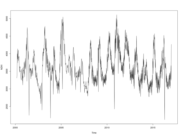
A visualization operation can be performed by creating an analogous function,
plot_ndvi_trend(). This plot_ndvi_trend() function operates similar to the
previously demonstrated get_ndvi_mean() function, except the
plot_ndvi_trend() function performs additional steps to ensure that the rows
are ordered chronologically and then it plots the data, returning a png image to
the SQL client in a similar way to that seen in earlier posts.
The average NDVI for San Diego county as a function of time can be determined
using the plot_ndvi_trend() function described above by executing the
following commands:
CREATE OR REPLACE FUNCTION plot_ndvi_trend(rastfile text)
RETURNS bytea AS $$
  library(cairoDevice)
  library(RGtk2)
  library(sp)
  library(raster)

  # prepare in-memory buffer for the image
  pixmap <- gdkPixmapNew(w=1024, h=768, depth=24); asCairoDevice(pixmap)

  # read preprocessed NDVI data
  ndvi <- brick(rastfile)

  # calculate layerwide-mean per layer
  ndvi_mn <- cellStats(ndvi, stat = 'mean')

  # read layer dates
  conn <- dbConnect(dbDriver("PostgreSQL"), user="postgres", dbname="gis", host="localhost")
  sql.str <- "SELECT lyr_date FROM ndvi_dates(get_robj('ndvi_dt'))"
  ndvi_dt <- dbGetQuery(conn, sql.str)

  # create vector index sorted by date
  idx <- order(ndvi_dt)

  # combine sorted vectors into a data.frame
  Data <- data.frame(ndvi_dt$lyr_date[idx], ndvi_mn[idx])

  # plot to the buffer
  plot(Data, type ="l", xlab = "Time", ylab = "NDVI")

  # capture and return the image to the client
  plot_pixbuf <- gdkPixbufGetFromDrawable(NULL, pixmap, pixmap$getColormap(),
                                          0, 0, 0, 0, 500, 500)
  gdkPixbufSaveToBufferv(plot_pixbuf, "png", character(0), character(0))$buffer
$$ LANGUAGE 'plr' STRICT;
The average NDVI for San Diego county as a function of time determined by the
plot_ndvi_trend() function can be returned as a png image to the SQL Client by
executing the following commands:
SELECT plr_get_raw(plot_ndvi_trend('/usr/local/bda/modis/ndvi_cooked/ndvi.tif'));
The graphical output for average NDVI over time is provided in Figure 1 below.

Figure 1: Average NDVI over time determined by plot_ndvi_trend() function
Visualize Average Over Time with ggplot
The average NDVI for San Diego county as a function of time can also be
visualized with an alternative plotting function called ggplot(). The
following pure R code will use this alternative plotting method to produce a png
image file:
library(sp)
library(raster)
library(ggplot2)
library(RPostgreSQL)

# might not be required depending on client setup
Sys.setenv("DISPLAY"=":0.0")

# read preprocessed NDVI data
ndvi <- brick(rastfile)
# calculate layerwide-mean per layer
ndvi_mn <- cellStats(ndvi, stat = 'mean')

# read layer dates
conn <- dbConnect(dbDriver("PostgreSQL"), user="postgres", dbname="gis", host="localhost")
sql.str <- "SELECT lyr_date FROM ndvi_dates(get_robj('ndvi_dt'))"
ndvi_dt <- dbGetQuery(conn, sql.str)

# create vector index sorted by date
idx <- order(ndvi_dt)

# combine sorted vectors into a data.frame
Data <- data.frame(ndvi_dt$lyr_date[idx], ndvi_mn[idx])

# use ggplot to create png file with the plot output
png("/tmp/ndvi_trend_gg.png", width = 1024, height = 768)
ggplot(Data, aes(x,y)) + geom_point() + geom_smooth()

# flush the output to file
dev.off()
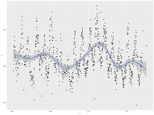
The graphical output for average NDVI for San Diego county over time visualized
using ggplot is provided in Figure 2 below.

Figure 2: Average NDVI over time visualized using ggplot
Note that the geom_smooth() argument to ggplot provided a nice regression
line with confidence bands. Various smoothing methods are available, but here we
have allowed ggplot to select the default. This addition aids the eye in
spotting trends in the data.
Visualize Average by Month
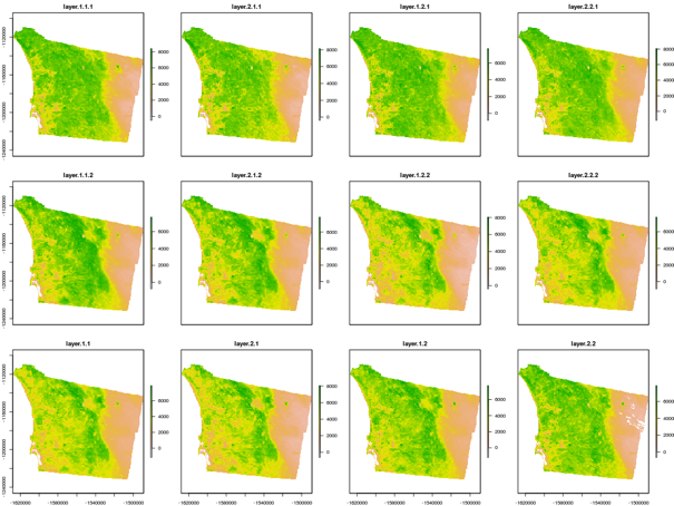
Using R commands, it is possible to create a visualization of the average NDVI for San Diego county by month for a given year. This visualization can be generated by executing the following commands:
plot_ndvi_year <- function(rastfile, layeryr, plotfile) {
  library(sp)
  library(raster)
  library(RPostgreSQL)

  Sys.setenv("DISPLAY"=":0.0")

  # required in R, noop in PL/R
  conn <- dbConnect(dbDriver("PostgreSQL"), user="postgres", dbname="gis", host="localhost")

  # plot to file if destination filename given
  if (plotfile != "") png(plotfile, width = 1024, height = 768)

  # read the dates
  conn <- dbConnect(dbDriver("PostgreSQL"), user="postgres", dbname="gis", host="localhost")
  sql.str <- "SELECT lyr_date FROM ndvi_dates(get_robj('ndvi_dt'))"
  ndvi_dt <- dbGetQuery(conn, sql.str)

  # read and plot requested raster layer
  ndvi <- brick(rastfile)
  ndvi_rast <- raster()

  # for each month and selected year, do pixel-wise aggregation to get one layer per month
  for (i in 1:12) {
    fmt_str <- paste(layeryr, sprintf("%02d", i), sep = "-")
    ndvi_layer <- mean(ndvi[[which(format(ndvi_dt, "%Y-%m") == fmt_str)]], na.rm = TRUE)
    ndvi_rast <- addLayer(ndvi_rast, ndvi_layer)
  }

  # plot and return
  plot(ndvi_rast)
  if (plotfile != "") dev.off()
}

plot_ndvi_year("/usr/local/bda/modis/ndvi_cooked/ndvi.tif", 2011, "/tmp/ndvi-2011.png")
It is worth noting that in this case, rather than averaging an entire raster layer to provide one NDVI value for the county, the commands are averaging pixel-by-pixel across multiple raster layers per month, in order to provide a composite image representing the given month. The visual output for average NDVI by month for the year 2011 is provided in Figure 3 below.

Figure 3: Visualization average NDVI for San Diego county by month
Visualize Same Month Average by Year
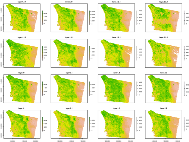
Using similar R commands, it is possible to create a visualization of the average NDVI for San Diego county for a given month, over a series of years.
plot_ndvi_month <- function(rastfile, layermonth, firstyr, lastyr, plotfile) {
  library(sp)
  library(raster)
  library(RPostgreSQL)

  Sys.setenv("DISPLAY"=":0.0")

  # required in R, noop in PL/R
  conn <- dbConnect(dbDriver("PostgreSQL"), user="postgres", dbname="gis", host="localhost")

  # plot to file if destination filename given
  if (plotfile != "") png(plotfile, width = 1024, height = 768)

  # read the dates
  conn <- dbConnect(dbDriver("PostgreSQL"), user="postgres", dbname="gis", host="localhost")
  sql.str <- "SELECT lyr_date FROM ndvi_dates(get_robj('ndvi_dt'))"
  ndvi_dt <- dbGetQuery(conn, sql.str)

  # read and plot requested raster layer
  ndvi <- brick(rastfile)
  ndvi_rast <- raster()

  # for each year and selected month, do pixel-wise aggregation to get one layer per month
  for (i in firstyr:lastyr) {
    fmt_str <- paste(i, sprintf("%02d", layermonth), sep = "-")
    ndvi_layer <- mean(ndvi[[which(format(ndvi_dt, "%Y-%m") == fmt_str)]], na.rm = TRUE)
    ndvi_rast <- addLayer(ndvi_rast, ndvi_layer)
  }

  plot(ndvi_rast)
  if (plotfile != "") dev.off()
}
The visual output for average NDVI for San Diego county for the month of January from 2001 to 2016 can be generated using the following command and is provided in Figure 4 below.
plot_ndvi_year("/usr/local/bda/modis/ndvi_cooked/ndvi.tif", 1, 2001, 2016, "/tmp/ndvi-1.png")

Figure 4: Visualization of average NDVI for San Diego county by month
Conclusion
While PostgreSQL is not necessarily known for use with analytic applications, the combination of PostgreSQL, PostGIS, PL/R and R provide PostgreSQL users with the combination of the power and efficiency of PostgreSQL and the rich analytic functionality of R. When further combined with PostGIS, the geospatial extender for PostgreSQL, users can perform powerful spatial analytics within the PostgreSQL database.
